Bertrand Model Example in Excel with Charts Download
The Bertrand model illustrates price competition in an oligopolistic market. It was formulated by the French mathematician and economist Joseph Bertrand in the late 19th century.
Bertrand described the behavior of firms that compete by adjusting the price of their product. He effectively depicted the consequences of price undercutting in a market economy.
Description of the Bertrand Financial Model
In the economic situation where two oligopolistic firms compete with each other, they reach a Nash equilibrium and end up making zero profit. This results in Bertrand's paradox.
In Bertrand's model, it is assumed that:
- There are at least two producers of homogeneous products in this market segment;
- Firms do not cooperate or collude;
- Marginal costs remain constant and are identical for both;
- Demand follows a linear function;
- Producers set prices simultaneously and independently;
- When the price is set, the quantity produced matches the demand;
- Consumers prefer cheaper goods;
- If prices are the same for both companies, their products are sold in equal shares;
- The model does not evolve but considers decisions at a specific moment in time.
In Bertrand's duopoly, a firm considers its competitor's price as constant. As the price of the competitor's product decreases, demand for it increases. Consequently, the company lowers its price, continuing until it equals the marginal costs.
Equilibrium is achieved at the level of perfect competition price.
Bertrand's Duopoly Model in Excel
Firm 1 sets a price for its product, P1. Firm 2, producing similar goods, has three options:
- Set a higher price (if P2 > P1, Firm 2 will not sell anything);
- Set the same price (if P2 = P1, both duopolists share market demand);
- Set a lower price to capture the entire market demand.
The third option is the most attractive, leading duopolists to act symmetrically. The strategy for each is to undercut the competitor's price, continuing until it matches average/marginal cost levels.
In the Bertrand model, sales volume is a function of price. The market demand equation looks like:
Q = a/b – 1/b*P
Producer costs are proportional:
TC1 = c * q1
TC2 = c * q2
Competitors lower their prices until they reach competitive equilibrium (price equals costs):
P* = MC = AC = c
The production volume for the first firm depends on the second firm's price:
- q1 = Q, if p1<p2;
- q1 = 0.5 Q, if p1=p2;
- q1 = 0, if p1>p2.
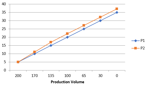
We will illustrate the production volume dependency on price using the Bertrand model on an Excel Chart.
Suppose the maximum demand for product X in a region is 200. A competitor sets a price of 20 for this product. We will create a table reflecting Firm 1's price formation.
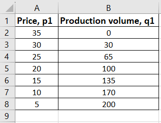
Maximum costs are 5. Firm 1 cannot go below this value; otherwise, it would operate at a loss.
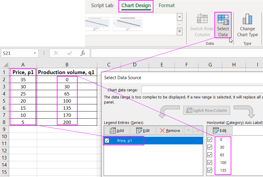
Demand follows a linear function. We plot the Chart by selecting "Insert" - "Charts." We then choose "Chart." The "Designer" tab becomes available, and we press "Select Data". On the x-axis, we have the production volume, and on the y-axis, the price.
We analyze the Chart:
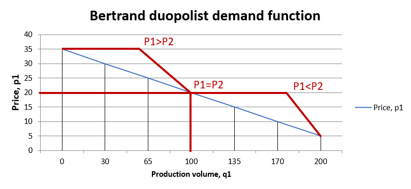
The maximum price set by the duopolist results in zero demand.
We will plot the reaction curves of firms producing homogeneous products. Firm 1 sets a slightly lower price than Firm 2.
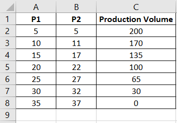
The reaction curves of firms run parallel to each other:
 Download Bertrand Model in Excel
The intersection point represents average costs. Neither competitor would set a price below this, as it would lead to production losses.
