Examples of using functions LARGE and SMALL in Excel
LARGE and SMALL functions in Excel are opposite in their meaning and are used to determine the largest and smallest numeric elements in the data set, respectively.
Note: In Excel, an array is a dataset represented as a single object (for example, a range of cells). An array in Excel can be taken as an argument.
Features conditions in the functions LARGE and SMALL
The functions LARGE and SMALL returns the kth maximum and minimum values, respectively, in the selected dataset. These functions are used to search for values that occupy a certain relative position in the data set.
Note: for a simple search for the smallest and largest values in a data range, it is customary to use the MIN and MAX functions, which take a single input parameter — the data range. LARGE and SMALL offer advanced functionality to search for the 1st, 2nd ... kth largest / smallest values in the array.
Both functions have similar syntax, so we will not consider it separately for each function. Consider the syntax for the LARGE:
=LARGE(array,k)
Argument Description:
- Array is a range or an array of numeric values for which the kth largest value is calculated. It is a required argument;
- K is an argument pointing to the position in the data set or array starting with the lowest value. It is also a required function argument.
Notes:
- If the value of the argument k exceeds the number of elements in the data array, is equal to zero, or is taken from a range of negative numbers, the result of the functions of the LARGE and SMALL will be the error #NUMBER!.
- Error #NUM! also occurs if the array is empty.
- The functions LARGE and SMALL ignore textual data that may be contained in an array.
- If, when using the LEASTING function as the argument k, to specify 1 (one), the result will be identical to the result of the MIN function;
- If, when using the SMALL as an argument k, specify the size of the array (the number of elements contained in it), the result will be identical to the result of the MAX function.
Examples of working in Excel with the functions of the LARGE and SMALL
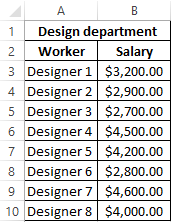
Example 1. In the design department of an enterprise 8 engineers work. It is necessary to determine the fourth largest and lowest wages, respectively.
Enter the data in the table:
To determine the lowest 4th salary in the department, we introduce the following formula in cell C2:
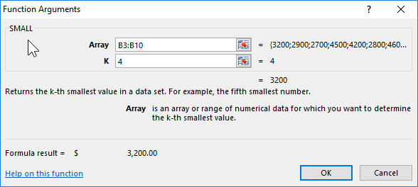
=SMALL(B3:B10,4)
The arguments of this function are:
- B3:B10 - an array of wage values for all employees;
- 4 - the order of the required smallest value in the array.
To determine the highest 4th salary, enter the formula in cell D2:
=LARGE(B3:B10,4)
The arguments of this function correspond to those that the SMALL function took in the context of this example.
We get the following results:
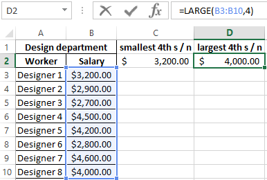
That is, the lowest and highest fourth wages in the department are equal to 3200 and 4000 monetary units, respectively.
Fourth smallest value in the array of numbers
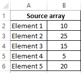
Example 2. For clarity of the function, we define the 1st, 2nd, 3rd, 4th and 5th elements of the data array, consisting of five elements. From the obtained results we will create a new table, thus performing, in fact, the sorting of the elements of the array in ascending order.
Enter the data in the table:
To solve, we will use the SMALL function, finding successively the smallest 1st, 2nd, ..., 5th values and entering them into the new table. For example, consider the process of finding the smallest 1st value. In cell C2, we introduce the following formula:
=SMALL(B2:B6,1)
The function takes the following arguments:
- B2:B6 - the range of values of the source array;
- 1 - the order of the smallest value.
In a similar way, fill the cells C3, C4, C5, and C6, indicating as the argument k the numbers 2, 3, 4, and 5, respectively.
As a result, we get:
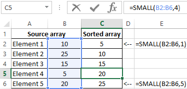
That is, we were able to sort the source array and clearly demonstrate the operation of the SMALL function.
Notes:
- In a similar way, you can reverse the sorting (from the largest to the smallest) using the LARGE function.
- It is better to use other Excel features for sorting, this example is provided only for the purpose of visual demonstration of work.
Formula of the functions is the LARGE with an array and sum
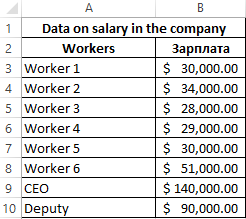
Example 3. The company employs 10 employees, including the CEO and his deputy. One of the employees suggested that both managers receive, in general, more than all other employees. It is necessary to determine whether this assumption is true or false.
We enter data on the salary of employees in the table:
It is obvious that the salary of any of the two managers is greater than that of any of the other employees. Therefore, we can use the LARGE function to find the salary values of the general director and the deputy. For the solution, we write the following formula:
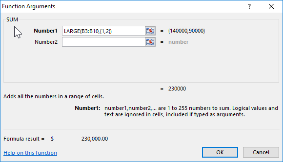
=SUM(LARGE(B3:B10,{1,2}))
The arguments to the SUM function are the values that the LARGE function returns. The latter takes the following arguments:
- B3:B10 - an array that stores data on the salaries of all employees of the company.
- {1,2} is the interval corresponding to the first and second desired quantities.
Note: {1,2} is a variant of writing arrays in Excel. With the help of this record it was indicated about the need to return the first two largest values from the array B3:B10. The resulting values will be summarized by the SUM function.
As a result, we get the amount of director and deputy salaries:
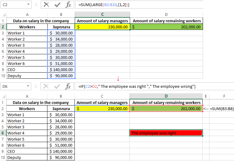
Now we determine the total amount of salaries of the remaining workers using the SUM function in cell D2.
Visually, the employee was right. However, we use Excel functionality to display the result of solving the problem in cell D6:
=IF(C2>D2," The employee was right "," The employee wrong")
The IF function takes the following arguments:
- C3>D3 is a logical expression, in which C3 is the cumulative salary of managers, D3 is the cumulative salary of the remaining employees;
- "The employee was right" - the text that will be displayed if C3>D3 is true;
- “The employee wrong” is the text that appears if C3>D3 is false.
Download examples using functions LARGE and SMALL in Excel
That is, both managers get more money than the rest of the staff combined.
