Example of how to use RAND and RANDBETWEEN functions in Excel

RAND and RANDBETWEEN have the same function - to generate random numbers. The result of the RAND function is a uniformly distributed random number (real), by default the range of such numbers is from 0 to 1. How Do Functions Work?



Random number generators RAND and RANDBETWEEN in Excel

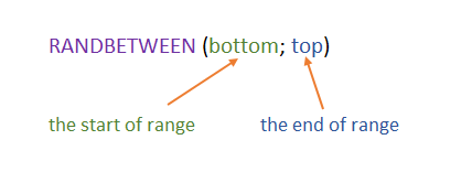
The syntax of such a function does not take any arguments. That is, it is not necessary to write anything inside the brackets, as we are already used to when working in Excel. RANDBETWEEN has the following syntax:

Let's start with the simplest first example, which will take up only one cell. In cell A1 we write the RAND function, we have no arguments in brackets and press Enter:

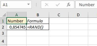
We got a random number in the range from 0 to 1. Now let's copy the formula down a few cells and see some feature in the work of RAND:

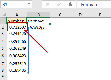
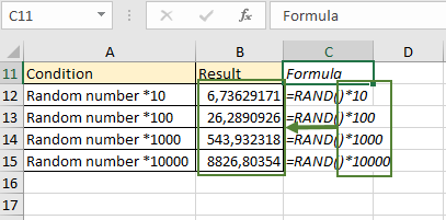
Note that the values in the first cell has changed. When we copied the function, the numbers were recalculated and new values were determined that correspond from 0 to 1. In the next example, we will look at how you can influence the returned result. Let's create a table in which we will determine some conditions. We can increment the return value. For instance, to get a number greater than 1, we add a multiplication by 10 to the RAND function:

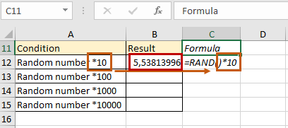
And so we change the value of the number as much as necessary. If you need two characters before the coma, multiply by 100 and so on. The same principle can be applied to the decimal fraction RANDBETWEEN function. Let's fill in our column:

If you need to limit the minimum and maximum value among a set of random numbers, then you need to use RANDBETWEEN. By setting the range limits, we get the generated numbers that do not go beyond the range:

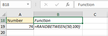
In the example, we specified the boundaries of the range as arguments. Now, the result corresponding to the conditions was returned. Copy the formula down to several cells:

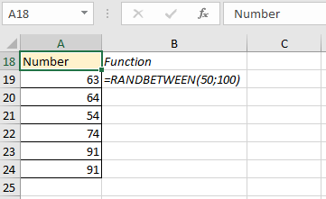
As you can see, all values are within the specified frames.



How to use RAND and RANDBETWEEN in practice?

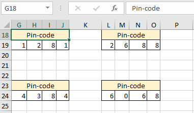
Where can such a simple and easy, seemingly incapable of significant calculations function be required? For example, when generating a PIN code. We have 4 cells, the boundaries for the RANDBETWEEN function will be 0 and 9. In cell G19, we write the formula and copy it in order:

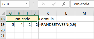
We have formed a 4-digit PIN code. But what if you need to get multiple random values for a PIN? Then you need to start recalculation. You can do this manually by pressing F9 on your keyboard. Now we have 4 fields with PIN codes with certain values:

Press F9 and see what result we have now:

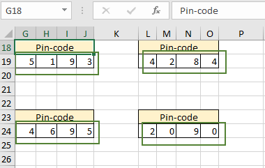
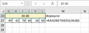
In all fields, in all cells, the values changed randomly. This can be done as many times as needed. Random number generation can also be used in different lotteries. For example, we have a range from 30 to 80, and we need to get 6 any numbers from this set. It is just as easy to complete this task - we specify “30” as the first argument for the function RANDBETWEEN, “80” as the second argument and copy for the next 5 cells:

We can also conclude that all tasks using the RANDBETWEEN function return a set of exclusively integer numbers. But how to solve the problem when you need results that are greater than 1, and a fractional remainder. We know that the RAND function partially fulfills this condition, since it returns the contents of the range from 0 to 1 with a fraction. And the RANDBETWEEN function fulfills the second of two conditions - you can specify the desired array. It turns out that you need to combine these two functions so that their joint calculation returns the desired result:

But now there is a small flaw in the formula. Let's recalculate the formula and take a closer look at the new values:

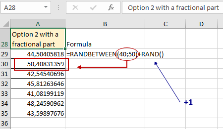
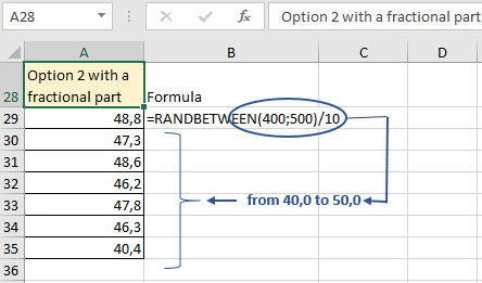
Now we can observe that we have a value that goes beyond the upper bound of the array. This is because RAND works according to the simple logic of mathematics and simply performs the specified addition operation - adding the generated fractional part to the upper bound. In order to avoid this disadvantage, you need to use a simple rule of mathematics. If you need fractional values from 40 to 50, then in the arguments for RANDBETWEEN we indicate the boundaries of 400 and 500 and divide the function by 10. Now we will return results from 40.0 to 50.0:

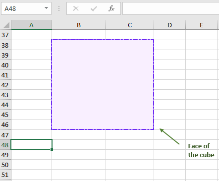
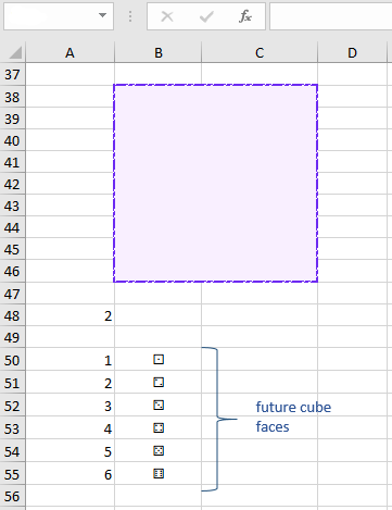
Having mastered the functions of generating random numbers, let's try to create a functional dice that can be used like a real one. Let's start by selecting and merging cells B38:C46. This will be our face of the cube. If you wish, you can add decorative effects, for example, make an unusual color frame and fill, preferably using a light background:

The address of this cell will be B38, because in the case of merging several cells, its address will be the upper leftmost cell before the merging. Later we will return to the square, but for now, we need to implement the main work of the die - "throw" the numbers from 1 to 6 in random order. In cell A48, start writing the formula:

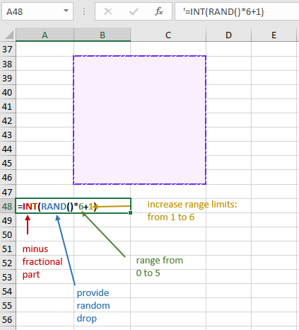
The way this formula works is as follows:

1. RAND will still generate numbers from 0 to 1 with a fraction.
2. The multiplication operation will change our range - it will turn out from 0.0 to 5.0.
3. We don't need a fraction, so we use an INT, in which we put a RAND with multiplication and addition. At this stage, we will get the range (0;5).
4. Add a unit to get the boundaries (1;6).

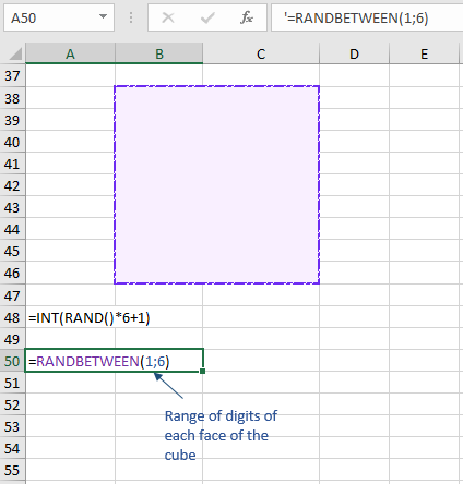
The same range can be obtained through RANDBETWEEN by simply specifying the desired boundaries:

We leave in cell A48 the option that we like best. To make the cube really look like a real one, we use the images of its faces, which we will add later to a large square. Cells A50:A55 will be filled with numbers from 1 to 6. Opposite the corresponding number, using Unicode characters, we will copy characters from the unicode-table.com resource to display all 6 faces:

Now we need to make sure that the “throw” of the die is displayed directly in cell B38. For this we created this large array. It is necessary to associate a randomly generated value from the RANDBETWEEN formula with the images of the face of the cube and the large cell B38. You can do this in several ways. The first is using the IF function. Since this formula has only two arguments, and we need to display 6 variations, we use the IF nesting property. In cell B38, enter the formula:

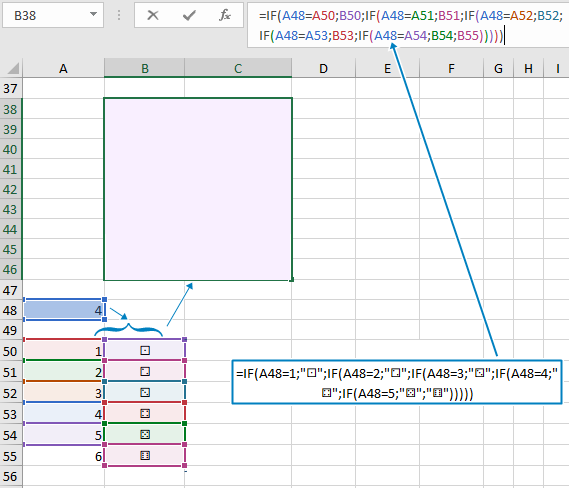
The principle of operation is simple: the first condition is checked and either cell B50 (value_if_true) is returned, or the transition to the “value_if_false” argument, which consists of a new IF with arguments and values. And so on the chain. Note that we don't use the sixth IF at the end, but just specify value_if_false for the fifth "IF" because that's the end of the chain and the sixth IF is not necessary. It is possible to use Unicode characters in the nested IF, which are represented by face images, instead of input addresses with face icons. There is another option for displaying the corresponding face. In cell C50, write the formula IF(A50=F$48;B50) and copy it up to cell C55 (the dollar symbol will ensure copying without unnecessary cell shifts). The formula checks if cell A50 contains the value from cell A48, then returns either a dice icon or empty text. After that, you need to provide a link between column C50:C55 and cube B38. To do this, you can use two options: either chain cells together using an ampersand, or through CONCATENATE, which performs the same option:

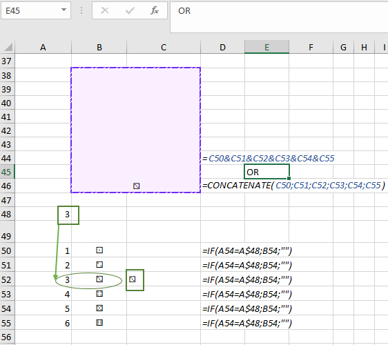
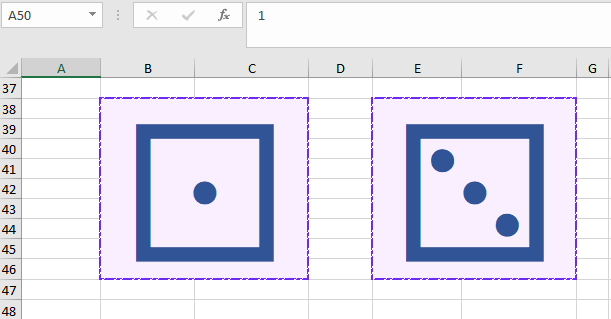
Both formulas from cells D44 and D46 work the same way: the concatenation of cells displays the text contained in them together, but since among these cells only one will always display a cube icon, and the other five will display empty text, the only unique one will be displayed in a large square icon. Now our cube is not looks exactly like the real one. In order to improve the graphic image, let's increase the text font of the cube in our case by 180. We can also change the color of the cube at will. If the game needs a pair of dice, just copy the entire array with the big square and the calculation array below, and place it next to the first one. Now we have two beautiful and functional dice. We can also continue to improve and hide all the calculations that are under the dice:

1. Select the entire range below the cubes.
2. On the "Home" tab, open a window in the "Number" subgroup.
3. Among the categories, select "all formats" and in the "Type" enter ;;; (three times dot with quotation mark).
4. Click "ok" and observe the final result:

Download examples of use RANDBETWEEN and RAND functions in Excel

In the cell A40 in the formula field, we still see that the text has not been removed but is hidden from view. To start a new "throw", it is enough to start the recalculation of functions - press the F9.